0/1 Knapsack Problem
Get started
জয় শ্রী রাম
🕉The knapsack problem is a combinatorial optimization problem that has many applications. In the knapsack problem, we have a set of items. Each item has a weight and a worth value. We want to put these items into a knapsack. However, it has a weight capacity limit. In our example below, the weight capacity is 15 kilogram. We cannot put any more than 15 kg of weight in the bag. Our objective is to choose the items in such a way so we get the most value. Therefore, we need to choose the items whose total weight does not exceed the weight capacity, and their total value is as high as possible. In the 0/1 knapsack problem, each item must either be chosen or left behind. We cannot take more than one instance for each item. You cannot take fractional quantity as well. That is why it is 0/1: you either take the whole item or you don't include it at all. For example, the best solution for the below example is to choose the 1kg, 1kg, 2kg item and 4kg item, which gives a maximum value of $15 within the weight capacity limit.

Many learners think 0/1 Knapsack Problem is scary. But it is NOT. It is super simple and having a command on the concept and implementation of 0/1 Knapsack will give you the upper hand while solving many complex looking Dynamic programming problems. Just by thinking logically can give you the solution to 0/1 Knapsack Problem.
-
What happens if weight of an item is larger than the weight capacity of the knapsack ?
We don't even consider including the item and move on to the next item. -
What happens if weight of an item is lower than the weight capacity of the knapsack ?
We have two options here: either include it or do not include it. And the onus of making the right decision is on you. So how do you decide whether to include the item or not? Simple! You calculate the max value you can get by including and not including the item. If including the item gives you more value then you decide to include the item. On the other hand, if excluding the item gives you more value, you then decide not to include the item.
Now it is very important to think through what are the implications of including or not including an item.- When we include an item the weight capacity of the knapsack goes down by the weight of the item. Next, we move to the next item.
-
When we do not include an item there is no change in knapsack weight capacity, and it remains
the same as it was when we reached the item.
We move to the next item with knapsack weight capacity unchanged.
The above discussion quickly gives us the recursion relationship for 0/1 Knapsack Problem:
Let's assume we have n items and W is the weight capacity of knapsack, and function dp(W, n) gives the max value that we can get when we have the knapsack with weight capacity W and all the items from index 1 to n (1-based index, NOT 0-based index, for discussion purpose; while writing code we would convert to 0-based index).
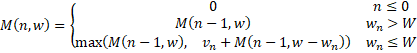
Notice that the base condition is: if given number of items is less than 1 then max value obtainable is 0 as it is not feasible to compute no item is given or negative number is provided for n.
Recursive Implementation:
Java code:
/**
 * Created by Abhishek on 1/2/21.
 */
public class Knapsack01 {
    int knapsackRecursive(int[] weight, int[] value, int n, int W) {
        if (n <= 0) {
            return 0;
        } else if (weight[n - 1] > W) { // weight of the item is greater than the weight capacity of the knapsack. Therefore do NOT include the item
            return knapsackRecursive(weight, value, n - 1, W);
        } else {
            return Math.max(knapsackRecursive(weight, value, n - 1, W), // do not include
                    value[n - 1] + knapsackRecursive(weight, value, n - 1, W - weight[n - 1])); // include
        }
    }

    public static void main(String[] args) {
        System.out.println(new Knapsack01().knapsackRecursive(new int[] {12, 2, 1, 4, 1}, new int[]{4, 2, 1, 10, 2},5,15)); // 15
        System.out.println(new Knapsack01().knapsackRecursive(new int[] {4, 5, 1}, new int[]{1, 2, 3},3,4)); // 3
        System.out.println(new Knapsack01().knapsackRecursive(new int[] {4, 5, 6}, new int[]{1, 2, 3},3,3)); // 0
    }
}
Python code:
class Knapsack01(object):
	# :type weight: List[int]
	# :type value: List[int]
	# :type n: int
	# :type W: int
	# :rtype: int
    def knapsackRecursive(self, weight, value, n, W):
        if n <= 0:
            return 0

        elif weight[n - 1] > W:
            #  weight of the item is greater than the weight capacity of the knapsack. Therefore do NOT include the item
            return self.knapsackRecursive(weight, value, n - 1, W)
        else:
            return max(self.knapsackRecursive(weight, value, n - 1, W), #do not include
            value[n - 1] + self.knapsackRecursive(weight, value, n - 1, W - weight[n - 1])) # include

kp01 = Knapsack01()
print(kp01.knapsackRecursive([12, 2, 1, 4, 1], [4, 2, 1, 10, 2], 5, 15)) #15
print(kp01.knapsackRecursive([4, 5, 1], [1, 2, 3], 3, 3)) #3
print(kp01.knapsackRecursive([4, 5, 6], [1, 2, 3], 3, 3)) #0
In each recursion step, we need to evaluate two sub-optimal solutions at max. Therefore, the running time of this recursive solution is O(2n).
Dynamic Programing Solution:
From recursion relation, we can quickly figure out an efficient bottom up (tabulation) Dynamic Programming approach.
Closely look: what all are the parameters change from one recursion call to another depending on what decision (to include an item or not to include) we take ? The index of the item (since after processing an item we move on to the next item) and the weight capacity of the knapsack. So n and W change.
So we would need a table of dimension n x W for sure with index (or number of items) on one axis and knapsack weight capacity on the other. Another way of determining it easily is to look at what are the parameters we need to pass to the recursion relation function at the minimum: we see it is n and W.
Optimal Substructure: In the recursive solution, notice that while computing result for higher degree of number of items we require result for lower degree of number of items. Same is true for knapsack weight capacity. So we should start computing from lower degree of n and W so that when we compute for higher degree of n and W, the result we are dependent on are already computed and ready to be reused. (BOTTOM-UP approach).
Note that we can achieve the same optimization by using Memoization along with recursion.
Java code:
int knapsackDP(int[] w, int[] v, int W) {
    int n = v.length;

    if (n <= 0 || W <= 0) {
        return 0;
    }

    int[][] m = new int[n + 1][W + 1];


    // m[0][j] = 0, for all j, since if there is zero item then we can get 0 max value
    // m[i][0] = 0, for all i, since if max weight limit is 0 then we get 0 max value

    for (int i = 1; i <= n; i++) {
        for (int j = 1; j <= W; j++) {
            if (w[i - 1] > j) {
                m[i][j] = m[i - 1][j];
            } else {
                m[i][j] = Math.max(
                  m[i - 1][j],
                  m[i - 1][j - w[i - 1]] + v[i - 1]);
            }
        }
    }
    return m[n][W];
}
Python code:
def knapsackDP(w, v, W):
        n = len(v)

        if n <= 0 or W <= 0:
            return 0

        m = [[0 for x in range(W + 1)] for y in range(n + 1)]
        #  m[i][j] gives
        #  m[0][j] = 0, for all j, since if there is zero item then we can get 0 max value
        #  m[i][0] = 0, for all i, since if max weight limit is 0 then we get 0 max value

        for i in range (1, n + 1):
            for j in range(1, W + 1):
                if w[i - 1] > j:
                    m[i][j] = m[i - 1][j]
                else:
                    m[i][j] = max(m[i - 1][j],
                              m[i - 1][j - w[i - 1]] + v[i - 1])

        return m[n][W]
Time Complexity: O(nW)
NOTE: Just for your knowledge, neither the recursive solution nor the above dynamic programming solution will scale for large number of items (>1000), because Knapsack is NP-complete. That running time of O(nW) hides an exponential nature.
O(n*W) looks like a polynomial time, but it is not, it is pseudo-polynomial.
What is very important to note is that Time complexity measures the time that an algorithm takes as a function of the length in bits of its input. The dynamic programming solution is indeed linear in the value of W, but exponential in the length of W — and that's what matters!
More precisely, the time complexity of the dynamic solution for the knapsack problem is basically given by a nested loop:
// here goes other stuff we don't care about
for (i = 1 to n)
    for (j = 1 to W)
        // here goes other stuff
What does it mean to increase linearly the size of the input of the algorithm? It means using progressively longer item arrays (so n, n+1, n+2, ...) and progressively longer W (so, if W is x bits long, after one step we use x+1 bits, then x+2 bits, ...). But the value of W grows exponentially with x, thus the algorithm is not really polynomial, it's exponential (but it looks like it is polynomial, hence the name: "pseudo-polynomial").
Let me shed more light on what I just said. When we say an algorithm is linear or O(n) we also mention n = size of the input array or list or whatever (depending on the problem at hand). So when an algorithm is linear it is actually linear in the size of the input and not linear to the input itself. The above algorithm is linear in the size of the of given items. But what makes it peudo-polynomial is the fact that it is also linear with value of weight limit W, which makes it exponential in size of W. Why ? Because size of an integer value is measured in bits. Like, size of 8 would be 4 since 8 = 2 3. 8 is represented as 10002 in binary system. So what do we get when number of bits increases from 3 to 4 ? We get 24 or 16. Let's see below how it increases with increase in number of bits:
25 < 26 < 27 < 28 and so on or, 32 < 64 < 128 < 256 and so on
So we see that the value is increasing exponentially as the size (i.e, number of bits) of the weight limit increases.
So in all, the time complexity is linear in the size of item array but exponential in the size of the weight limit of knapsack. Therefore, the time complexity is 'pseudo-polynomial'.
To scale out, we need to use a constraint solver, such as OptaPlanner (Java open source) that uses more appropriate algorithms for a much larger scale, such as Late acceptance, Tabu Search or Simulated Annealing.
Space Optimization:
In the previous solution, we used a n * W matrix. We can reduce the used extra space. Look how at every iteration we are using values from the same row and the row above. So at any point of time while computing for row i if we only keep the value for row (i - 1), that should be enough, which means at any point of time we only need 2 rows: row i and row (i - 1).
So what we can do is, we can take a 2-D array dp[][] with just 2 rows, and for all rows with odd index, like index = 1, 3, and so on, we store the values in dp[1], and for all rows with even indices we store values in dp[0].
If n is odd, then the final answer will be at dp[0][W] and if n is even then the final answer will be at dp[1][W] because index starts from 0.
Please see the code below and the concept will become clear.
Login to Access Content
Further Optimization:
We can do further space optimization.
The code above is O(2 * W) = O(W), since we still used 2D array and not an 1D array. Here we will be solving the problem by using 1D array.
If you look closely, we need two values from the previous iteration: dp[w] and dp[w - weight[i]]
Since in our inner loop w is iterating from 0 to max weight limit W, let’s see how this might affect our two required values:
- When we access dp[w], it has not been overridden yet for the current iteration, so it should be fine.
- dp[w - weight[i]] might be overridden if “w - weight[i] > 0”. Therefore we can’t use this value for the current iteration.
To solve the second case, we can change our inner loop to process in the reverse direction: iterating w from W to 0, something like below:
// iterate through all items
for(int i = 0; i < n; i++)  {
    //traverse dp array from right to left
    for(int j = W; j >= wt[i]; j--) {
        dp[j] = Math.max(dp[j] , val[i] + dp[j - wt[i]]);
    }
}
This will ensure that whenever we change a value in dp[], we will not need it anymore in the current iteration.
Below is the complete implementation:
Java code:
Login to Access Content
Python code:
Login to Access Content
Summary:
-
Most problems where you need to make up a target sum using at most one instance of each of the given items, can be solved using 0/1 Knapsack concept.